Reading data to analyse in memory

It’s often quickest and easiest to load data into memory before analysing it.

Some types of data, especially from large pixel detectors, may be bigger than the available memory. Other examples show how to work with very large amounts of data. But the machines in the Maxwell cluster have 250–750 GB of memory, so you can use the simple approach for many cases.

[1]:

%matplotlib inline
import matplotlib.pyplot as plt
import numpy as np
import re
import xarray as xr

from extra_data import open_run

Tabular data (with pandas)

We can open a run with EXtra-data on the Maxwell cluster using the proposal & run number.

[2]:

run = open_run(proposal=900025, run=150)
run.info()  # Show overview info about this data

# of trains:    3721
Duration:       0:06:12.1
First train ID: 142844490
Last train ID:  142848210

0 detector modules ()

2 instrument sources (excluding detectors):
  - SA1_XTD2_XGM/XGM/DOOCS:output
  - SPB_XTD9_XGM/XGM/DOOCS:output

2 control sources:
  - SA1_XTD2_XGM/XGM/DOOCS
  - SPB_XTD9_XGM/XGM/DOOCS

This example works with data from two X-Ray Gas Monitors (XGMs). These measure properties of the X-ray beam in different parts of the tunnel. This data refers to one XGM in XTD2 and one in XTD9.

pandas is a popular Python library for working with tabular data. We’ll create a pandas dataframe containing the beam x and y position at each XGM, and the photon flux. We can select the columns using ‘glob’ patterns, like selecting files in the terminal.

[abc]: one character, a/b/c
?: any one character
*: any sequence of characters

[3]:

df = run.select([("*_XGM/*", "*.i[xy]Pos"), ("*_XGM/*", "*.photonFlux")]).get_dataframe()
df.head()

[3]:

	SPB_XTD9_XGM/XGM/DOOCS/beamPosition.iyPos	SPB_XTD9_XGM/XGM/DOOCS/pulseEnergy.photonFlux	SPB_XTD9_XGM/XGM/DOOCS/beamPosition.ixPos	SA1_XTD2_XGM/XGM/DOOCS/beamPosition.iyPos	SA1_XTD2_XGM/XGM/DOOCS/pulseEnergy.photonFlux	SA1_XTD2_XGM/XGM/DOOCS/beamPosition.ixPos
trainId
142844490	1.717195	1327.06958	-2.277912	0.161399	1410.723755	2.035218
142844491	1.717195	1327.06958	-2.277912	0.161399	1410.137451	2.035218
142844492	1.717195	1327.06958	-2.277912	0.161399	1410.137451	2.035218
142844493	1.717195	1327.06958	-2.277912	0.161399	1410.137451	2.035218
142844494	1.717195	1327.06958	-2.277912	0.161399	1410.137451	2.035218

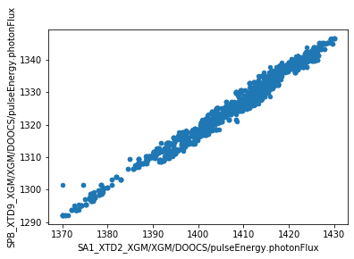
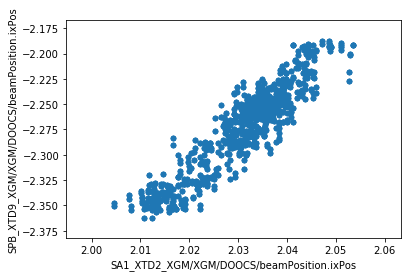
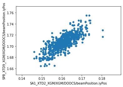
We can now make plots to compare the parameters at the two XGM positions. As expected, there’s a strong correlation for each parameter.

[4]:

df.plot.scatter(
    x='SA1_XTD2_XGM/XGM/DOOCS/pulseEnergy.photonFlux',
    y='SPB_XTD9_XGM/XGM/DOOCS/pulseEnergy.photonFlux',
)

[4]:

<matplotlib.axes._subplots.AxesSubplot at 0x2ba7e87f8fd0>

[5]:

ax = df.plot.scatter(
    x='SA1_XTD2_XGM/XGM/DOOCS/beamPosition.ixPos',
    y='SPB_XTD9_XGM/XGM/DOOCS/beamPosition.ixPos',
)

[6]:

ay = df.plot.scatter(
    x='SA1_XTD2_XGM/XGM/DOOCS/beamPosition.iyPos',
    y='SPB_XTD9_XGM/XGM/DOOCS/beamPosition.iyPos',
)

We can also export the dataframe to a CSV file - or any other format pandas supports - for further analysis with other tools.

[7]:

df.to_csv('xtd2_xtd9_xgm_r150.csv')

As arrays (with xarray)

We’ll open a different run for this example:

[8]:

run = open_run(proposal=900027, run=67)
run.info()  # Show overview info about the data

# of trains:    1475
Duration:       0:02:27.5
First train ID: 128146446
Last train ID:  128147920

0 detector modules ()

1 instrument sources (excluding detectors):
  - SA3_XTD10_PES/ADC/1:network

11 control sources:
  - SA3_XTD10_PES/ADC/1
  - SA3_XTD10_PES/ASENS/MAGN_X
  - SA3_XTD10_PES/ASENS/MAGN_Y
  - SA3_XTD10_PES/ASENS/MAGN_Z
  - SA3_XTD10_PES/DCTRL/V30300S_NITROGEN
  - SA3_XTD10_PES/DCTRL/V30310S_NEON
  - SA3_XTD10_PES/DCTRL/V30320S_KRYPTON
  - SA3_XTD10_PES/DCTRL/V30330S_XENON
  - SA3_XTD10_PES/GAUGE/G30300F
  - SA3_XTD10_PES/GAUGE/G30310F
  - SA3_XTD10_PES/MCPS/MPOD

This run includes data from a Photo-Electron Spectrometer (PES), a monitoring device which records energy spectra for each train. Here’s the data from one of its 16 spectrometers:

[9]:

run['SA3_XTD10_PES/ADC/1:network', 'digitizers.channel_4_A.raw.samples'].xarray()

[9]:

<xarray.DataArray 'SA3_XTD10_PES/ADC/1:network.digitizers.channel_4_A.raw.samples' (trainId: 1475, dim_0: 40000)>
array([[ -6, -10,  -7, ..., -10,  -8,  -9],
       [ -8,  -8,  -7, ...,  -9,  -2, -11],
       [ -8, -10,  -7, ...,  -6,  -8, -11],
       ...,
       [ -7,  -9,  -8, ...,  -9,  -2,  -5],
       [ -5, -10,  -8, ...,  -5,  -4, -10],
       [ -7,  -8,  -7, ...,  -6,  -5,  -8]], dtype=int16)
Coordinates:
  * trainId  (trainId) uint64 128146446 128146447 ... 128147919 128147920
Dimensions without coordinates: dim_0

The PES consists of 16 spectrometers arranged in a circle around the beamline. We’ll retrieve the data for two of these, separated by 90°. N and E refer to their positions in the circle, although these are not literally North and East.

xarray extends numpy arrays with metadata about the dimensions: we use this to annotate the data with the pulse train IDs they relate to. This is important when correlating data from different sources, as each source may be missing data for some pulse trains, so we need to match them up based on train IDs. See the page on Aligning data from different sources for more about this.

[10]:

data_n = run['SA3_XTD10_PES/ADC/1:network', 'digitizers.channel_4_A.raw.samples'].xarray()
data_e = run['SA3_XTD10_PES/ADC/1:network', 'digitizers.channel_3_A.raw.samples'].xarray()

data_n, data_e = xr.align(data_n, data_e)
nsamples = data_n.shape[1]
data_n.shape

[10]:

(1475, 40000)

We’ll get a few other values from the run to annotate the plot. This uses pandas - see the section above for more about that.

[11]:

# Get the first values from four channels measuring voltage
electr = run.select('SA3_XTD10_PES/MCPS/MPOD', 'channels.U20[0123].measurementSenseVoltage').get_dataframe()
electr_voltages = electr.iloc[0].sort_index()
electr_voltages

[11]:

SA3_XTD10_PES/MCPS/MPOD/channels.U200.measurementSenseVoltage   -0.101792
SA3_XTD10_PES/MCPS/MPOD/channels.U201.measurementSenseVoltage   -0.111782
SA3_XTD10_PES/MCPS/MPOD/channels.U202.measurementSenseVoltage   -0.106823
SA3_XTD10_PES/MCPS/MPOD/channels.U203.measurementSenseVoltage   -0.107910
Name: 128146446, dtype: float32

[12]:

gas_interlocks = run.select('SA3_XTD10_PES/DCTRL/*', 'interlock.AActionState').get_dataframe()

# Take the first row of the gas interlock data and find which gas was unlocked
row = gas_interlocks.iloc[0].sort_index()
print(row)
if (row == 0).any():
    key = row[row == 0].index[0]
    target_gas = re.search(r'(XENON|KRYPTON|NITROGEN|NEON)', key).group(1).title()
else:
    target_gas = 'No gas'

SA3_XTD10_PES/DCTRL/V30300S_NITROGEN/interlock.AActionState    1
SA3_XTD10_PES/DCTRL/V30310S_NEON/interlock.AActionState        0
SA3_XTD10_PES/DCTRL/V30320S_KRYPTON/interlock.AActionState     1
SA3_XTD10_PES/DCTRL/V30330S_XENON/interlock.AActionState       1
Name: 128146446, dtype: uint32

Now we can average the spectra across the trains in this run, and plot them.

[13]:

x = np.linspace(0, 0.0005*nsamples, nsamples, endpoint=False)

fig, axes = plt.subplots(1, 2, figsize=(10, 4))
for ax, dataset, start_time in zip(axes, [data_n, data_e], [15.76439411, 15.76289411]):
    ax.plot(x, dataset.sum(axis=0))
    ax.yaxis.major.formatter.set_powerlimits((0, 0))
    ax.set_xlim(15.75, 15.85)
    ax.set_xlabel('time ($\mu$s)')

    ax.axvline(start_time, color='red', linestyle='dotted', label='Start time')
    ax.axvline(start_time + 0.0079, color='magenta', linestyle='dotted', label='Neon K 1s')
    ax.axvline(start_time + 0.041, color='black', label='Auger peak')
    ax.legend()

axes[0].set_title('Spectrometer 00 N')
axes[1].set_title('Spectrometer 04 E')
fig.suptitle('{gas};  900 eV; [A B C D] = [{voltages[0]:.1f} {voltages[1]:.1f} {voltages[2]:.1f} {voltages[3]:.1f}] V; run 67'
             .format(gas=target_gas, voltages=electr_voltages.values), y=1.05);

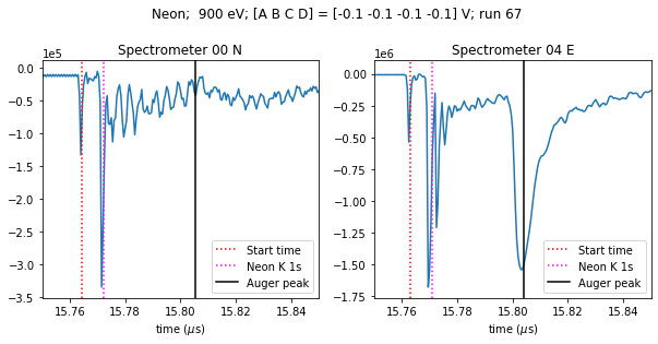
The spectra look different because the beam is horizontally polarised, so the E spectrometer sees a peak that the N spectrometer doesn’t.